Physical Stratigraphy

Stratigraphy is the area of geology devoted to the study of rock layers (strata), typically in sedimentary and volcanic rock units. Different rock types (lithologies) of an area may be described, interpreted, and even correlated with similar rocks in other locations.


Figure 5-16. Stratigraphy in the Grand Canyon.

Stratigraphic Columns

Stratigraphic columns are vertical sequences of rocks that represent an area's geologic history. Any single column can be read vertically, with lower units representing older events and higher units representing younger events (remember Superposition?). The lithology of the different rock units can be represented by certain pattern fills (see Figure 5-17). Resistant, cliff-forming units can also be drawn with near-vertical profiles, whereas softer, slope-forming units have more slanted profiles (see Figures 5-17 and 5-18).

W&M strat column

Figure 5-17. A simplified stratigraphic column with unit names.

See the Key to Fill Patterns for Rock Units PDF HERE for the list of standardized fill patterns.

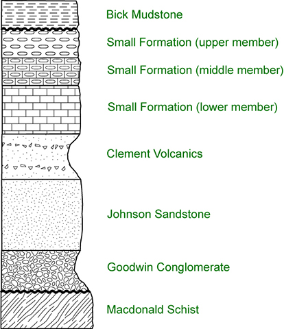
Let's review by looking at the strat column in Figure 5-17.

> The eight separate lithologic units each have a distinctive fill pattern. For example, the dotted pattern represents sandstone, the brick pattern represents limestone, etc.

> The Small Formation is composed of three seperate members, each having slightly different compositions.

> Volcanic ash layers (like the Clement Volcanics) typically make good markers beds because they can be deposited over large geographic areas and may also be datable (they are igneous in origin and may have datable isotopic content). These can be used to correlate startigraphic columns separated by large distances.

> Unconformities, like the one between the Macdonald Schist and Goodwin Conglomerate, are drawn with squiggly, bolded lines (thicker than normal unit contacts).

> Resistant, cliff-forming units are represented by near-vertical profiles (like the Johnson Sandstone), whereas softer, slope-forming units are represented by more slanted profiles (like the Goodwin Conglomerate).

> The formation names are in honor of my five undergraduate geology professors at William and Mary :)

Now let's try to interpret a geologic history from the stratigraphic column in Figure 5-17. We will start with the lowest sedimentary layer (the Goodwin Conglomerate) and work our way upwards through the section. We will successively interpret the depositional conditions and environment for each unit and then put it all together in the end.

Example 5

A possible interpretation of the stratigraphic column in Figure 5-17.

Time 1

The conglomerate is deposited over the schist in a high-energy nearshore environment (beach).

A nonconformity is thus formed between the two units.

Time 2

Rising sea level causes deposition of shallow marine sand over the beach conglomerate.

Time 3

A large nearby eruption deposits a layer of volcanic ash over the sandstone.

Time 4

Calcareous sediment is deposited as sea level rises and water depth increases.

Time 5

Cherty-calcareous sediment is deposited as water depth continues to increase.

The chert suggests a change from a shallow marine environment to deeper marine environment.

Time 6

Chert is deposited as water depth continues to increase.

At this point, the shoreline is furthest from the strat section location.

Time 6-7

A period of uplift and erosion occurs.

Time 7

Mudstone of flood-plain origin is deposited over the chert.

A disconformity is thus formed between the two units.

Overall

A marine transgression (rising sea level with the shoreline moving inland) occurred as several marine units of progressively deeper marine origin were deposited.

A brief period of volcanism occurred during this process.

This rise in sea level was followed by a marine regression (falling sea level with the shoreline moving seaward), where uplift and erosion of the marine units occurred.

This was followed by deposition of the flood plain mudstone, creating the disconformity.

Stratigraphic Correlation

Correlation of rock units across large areas typically yields a more complete understanding of the geologic history of a region and involves comparison of various characteristics (composition, thickness, age, etc.) of rock units from one place to another. If rock units are suitably exposed, their contacts can be traced across an area (either on foot or with aerial imagery). Isolated rock units can be correlated based upon distinguishing lithologic characteristics, like color, composition, sedimentary structures, fossils, etc. Buried rock units can sometimes be correlated using well data or geophysical methods. Thus, rocks in one area can be compared to rocks in other areas.

Many rock units display remarkably little relative change in lithology across wide areas, and thus are good for correlation purposes. One example is the Coconino Sandstone, which changes little from Sedona to the Grand Canyon. Another example of a rock type that is commonly excellent for correlation is tuff (volcanic ash), which may show little variation in composition or thickness over wide areas. This type of distinctive unit is called a marker bed or marker unit. Ash tuff commonly can be isotopically dated as well.

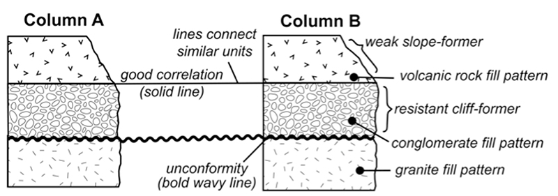
Correlation of stratigraphic columns from different areas can show variations in the composition, thickness, and relative order of rock types across a region. Thus, a series of stratigraphic columns can yield a wealth of information about the geology across a region over a certain interval of time. Figure 5-18 shows three units that are correlated between columns A and B. This is done by using straight lines to connect the upper and lower contacts of the rock unit with the same contacts of the rock unit in the other column. Each unit in Column A directly correlates with the same lithologies in Column B. A solid line is drawn if the correlation is convincing. Unconformities between rock units are drawn with squiggly, bolded lines (thicker than normal unit contacts). Figure 5-18 shows a nonconformity between the granite and conglomerate. These can also be correlated between strat columns.

Strat columns

Figure 5-18. Simplified stratigraphic columns and their correlation.

Difficulties Encountered in Correlation

Many rock units are not originally widely deposited, and only exist in local areas. Even if rock layers extend across large areas, it is more the exception than the rule for rock units to remain the same in lithology and/or thickness. A change in the lithology of a rock unit from place to place may be described as a facies change, which is caused as depositional characteristics change with distance and time. For example, mud deposited on a river flood plain relatively close to the active channel is likely to contain more sand than if it was deposited farther from the channel. Facies changes may involve a complete change in lithology (e.g. from sandstone to limestone) or only minor lithologic changes in the same unit (e.g., between a limestone to a cherty limestone). An Arizona example of a facies change is provided by the Moenkopi Formation, which changes from a thick sequence (more than 2000 feet) of dominantly marine limestone in southern Nevada to a much thinner sequence (less than 500 feet) of flood plain mudstone in northern Arizona.

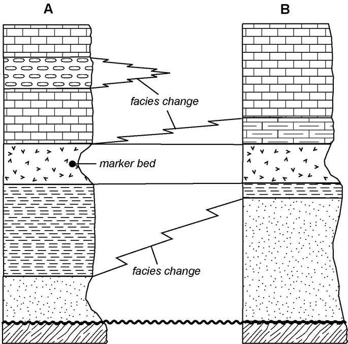
Facies changes of rock units are shown as saw tooth lines that represent the changes in lithology within the same unit from one column to another. Figure 5-19 displays a lateral facies change exists where rock units present in one column are much thinner or missing in the adjacent column. The contacts of a unit that "pinches out are drawn as converging saw tooth lines that meet between the two columns.

Other problems encountered in correlation are the lack of suitable rock outcrops and structural deformation. Rocks are commonly covered by soil or vegetation, and if rock layers are highly folded or faulted, then correlation becomes progressively more difficult.

Strat column facies changes

Figure 5-19. Facies changes in stratigraphic columns.

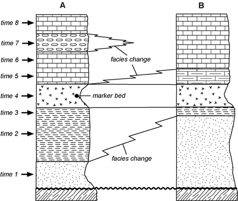
Now let's try to interpret a geologic history from the two correlated stratigraphic columns shown in Figure 5-19. We will proceed as we did in the previous example, starting with the lowest sedimentary layer and working our way upwards through the section. We will successively interpret the depositional conditions and environment and then put it all together in the end

Example 6

A simple interpretation of Columns A and B in Figure 5-19.

Example 06 strat column

Time 1

Shallow marine sand is deposited over schist at both A and B, creating a nonconformity (rising sea level causes the ocean to flood the land).

Time 2

Marine mud deposited at A, while sand still deposited at B.

This facies change between A and B may be due to:

1) greater water depth at A than at B or 2) A may be farther from land than at B or 3) both.

Time 3

Marine mud deposited at both A and B (similar depositional conditions at both A and B).

Time 4

Volcanic ash deposited at both A and B (the ash forms a marker bed).

Time 5

Muddy calcareous sediment deposited at B, while only calcareous sediment deposited at A.

This facies change between A and B may be due to

1) greater water depth may be at A than at B or 2) A may be farther from land than at B or 3) both).

Time 6

Calcareous sediment is deposited at both A and B (similar depositional conditions at both A and B).

Time 7

Chert deposited at A, while calcareous sediment is deposited at B (deeper water at A than at B).

Time 8

Calcareous sediment is deposited at both A and B (similar depositional conditions at both A and B).

Overall

A marine transgression occurred at A and B, with A representing deeper water farther from the shoreline.

You're Becoming a Stratigrapher!

Quiz Me! questions D46 through D50 refer to the stratigraphic columns shown in Figure 5-20. Click HERE to refer to a printable hard-copy PDF version of the fill pattern chart. Also refer to the Sedimentary Rock Identification Chart HERE for information about depositional environments for various rock types.